Analyzing Pathways from PTMs: A Guide

Purpose

This vignette intends to help users produce a matrix with PTM names as row names (e.g. FYN p Y411) and numeric data in all the columns, which can be used as input to the PTMsToPathways functions.

Mass spectrometry data output will vary depending on the experimental design, source of data, and software used to process the raw spectra. R supports many file types and can automatically convert them into a data frame. For example, read.csv() will take a csv file and convert it into a data frame (read.csv() is a variation of read.table()). We start with data in tab-delimited spreadsheet format.

Naming conventions

In this vignette, we use the following shorthand conventions when describing PTMs based on the modifications present in the example data set. Your data will dictate the names of modifications.

Gene.Name = The HUGO Gene Name is used to identify the protein/gene
Phosphorylation = “p”
Lysine acetylation = “ack”
Lysine methylation = “kme”
Arginine methylation = “rme”
Ubiquitination = “ubi”

Data input

Investigators will need to identify which columns contain key information for analysis of PTMs. The example raw data file for this vignette (downloadable here, or load directly into R using the commands below) contains only phosphorylation sites.

“Amino Acid” has the modified amino acid, e.g. S,T, etc.
“Positions Within Proteins” is the amino acid number in the protein sequence.
Ambiguous modification sites (a modification site whose peptide sequence is the same in more than one protein) have multiple possible postions separated by “;”.
“Modification Type” has Phosphorylation” etc.

Note that R converts spaces in column names to periods. After reading in our data table, the relevant column names are:

genes = “AllGeneSymbols”

positions = “Positions.Within.Proteins”

aa = “Amino.Acid”

modification = “Modification.Type”

We provide a helper function name.peptide() to make a PTM name using these columns. This function concatenates ambiguous modification sites and ignores NA values that are present in cells or ambiguous gene names.

Note that it is very important that the rownames are the names of post-translational modifications. All of their respective columns are the experimental conditions under which the post-translational modifications occurred. The numeric values are data output by the mass spectrometer. NAs – which are importantly not zeroes – represent missing data. Ambigious PTMs, cases where a PTM could be any one of several PTMs, are separated by semicolons. (e.g. “AARS ubi k747; AMBLIL p U123”).

Many investigators will examine their data in Microsoft Excel, which can export the spreadsheet in tab- or comma-delimited format. Unfortunately, Excel inescapably turns some gene names into dates when present in a cell by themselves. We reverse this with an example helper function, fix.excel():

fix.excel <- function(cell) {
  fixgenes = c("CDC2", "1-Sep", "2-Sep", "3-Sep", "4-Sep", "5-Sep", "7-Sep",
               "8-Sep", "9-Sep", "10-Sep", "11-Sep", "15-Sep", "6-Sep", "1-Oct",
               "2-Oct", "3-Oct", "4-Oct", "6-Oct", "7-Oct", "11-Oct", "1-Mar",
               "2-Mar", "3-Mar", "4-Mar", "5-Mar", "6-Mar", "7-Mar", "8-Mar",
               "9-Mar", "10-Mar", "11-Mar", "C11orf58", 'C17orf57', 'C3orf10',
               'C7orf51', "C11orf59", "C4orf16", "1-Dec", "14-Sep")
  
  corrects = c("CDK1", "SEPT1", "SEPT2", "SEPT3", "SEPT4", "SEPT5", "SEPT7",
               "SEPT8", "SEPT9", "SEPT10", "SEPT11", "SEPT15", "SEPT6",
               "POU2F1", "POU2F2", "POU5F1", "POU5F1", "POU3F1", "POU3F2",
               "POU2F3", "MARCH1", "MARCH2", "MARCH3", "MARCH4", "MARCH5",
               "MARCH6", "MARCH7", "MARCH8", "MARCH9", "MARCH10", "MARCH11",
               "SMAP", "EFCAB13", "BRK1", "NYAP1", "LAMTOR1", 'AP1AR', "DEC1",
               "SEPT14")
  
  cellv <- unlist(strsplit(as.character(cell), "; "))
  
  if (any(fixgenes %in% cellv)) {
    
    cellv.new <- gsub(fixgenes[fixgenes %in% cellv],
                      corrects[fixgenes %in% cellv], cellv)
    return (paste(cellv.new, collapse="; "))
    
  } else return(cell)
  }

We provide another example helper function, name.peptide(), to handle ambiguous modification sites (a modification site whose peptide sequence is the same in more than one protein) separated by “;” or another separator.

name.peptide <- function (genes, modification="p", sites, aa, pepsep=";")   {
  genes.v <- unlist(strsplit(genes, pepsep, fixed = TRUE))
  genes.v[which(genes.v == "NA")] <- NA
  genes.v <- genes.v[!is.na(genes.v)]
  
  sites.v <- unlist(strsplit(sites, pepsep, fixed = TRUE))
  sites.v[which(sites.v == "NA")] <- NA
  sites.v <- sites.v[!is.na(sites.v)]
  sites.v <- sapply(sites.v, function (x) paste (aa, x, sep=""))
  
  Peptide.v <- as.character(noquote(paste(
    genes.v[1:length(genes.v)], modification,
    sites.v[1:length(sites.v)], sep=" ")))
  
  Peptide <- paste(unique(Peptide.v), collapse="; ")
  
  return(Peptide)
}

Read in data file that is output from mass spectrometry. If you have installed the PTMsToPathways package, you can use the example data file included in the package as below. To use your own data file, replace file_path variable with your own path to file, as in the commented line below.

# file_path <- "path/to/your/file.txt"
file_path <- system.file("extdata", "phospho_cleaned_mapped.txt",
                         package = "PTMsToPathways")

newphos <- read.table(file_path, sep = "\t", skip = 0, header = TRUE,
                      blank.lines.skip = T, fill = T, quote = "\"", dec = ".",
                      comment.char = "", stringsAsFactors = F)
dim(newphos)
>> [1] 933 170

First remove internal control rows (reverse sequences).

newphos <- newphos[!is.na(newphos$AllGeneSymbols),]
dim(newphos)
>> [1] 908 170

If there are dates in the AllGeneSymbols column, use:

newphos$AllGeneSymbols <- sapply(newphos$AllGeneSymbols, fix.excel)

Next, identify the columns that will be used to name the PTM

headercols <- c("AllGeneSymbols", "Amino.Acid",
                "Positions.Within.Proteins", "Modification.Type")

Make a separate data frame using these columns.

newphos.head <- newphos[,headercols]

Now create a unique PTM name (peptide name)

newphos.head$Peptide.Name <- mapply(
  name.peptide, genes = newphos.head$AllGeneSymbols,
  sites =  newphos.head$Positions.Within.Proteins, aa = newphos.head$Amino.Acid)

Replacing Patterns

If the list of PTMs possesses symbols that are unnecessary such as “AARS ~K ubi K747”, this command will remove all strings included in the “patterns” vector from the rownames. Any pattern can be chosen so long as the user ensures that any special character (such as $ or @) have a “\” in front of them.

patterns <- c("\\~", "\\#", "/", "\\$", "\\@", "\\|")
patterns <- patterns[order(nchar(patterns), patterns, decreasing = TRUE)]

rownames(newphos) <- sapply(rownames(newphos), function(x){
  for(p in patterns) x <- gsub(p, "", x); return(x)
  })

Data columns

Next we identify the data columns, which contain the string “Intensity.” The example data file is from a multi-PTM study and the data in this table are from just the phosphorylation pulldown (other tables are for other PTM types). The optimal pulldown columns are straightforward to identify by the pulldown strings present in the sample names, “pTyr” in this case. They are also identifiable by zooming out and looking at the patterns of missing data, the optimal pulldowns, as a group, have the least missing data. The second step is to select colums that have “pTyr.”

These data have technical replicates, which means that the same samples were run twice. Due to the stochastic selection of peptides for detection, the pattern of missing values is slightly different between technical replicates. We therefore merge the technical replicates taking the value of either replicate where it’s missing in the other, and averaging values detected in both, using the function, merge2cols().

Key for column names

C = Crizotinib

D = DMSO

E = Erlotinib

Pr = PR171

For Intensity columns

C1-1: Crizotinib biological replicate 1- technical replicate 1

C1-2: Crizotinib biological replicate 1- technical replicate 2

C2-1: Crizotinib biological replicate 2- technical replicate 1

C2-2: Crizotinib biological replicate 2- technical replicate 2

C3-1: Crizotinib biological replicate 3- technical replicate 1

C3-2: Crizotinib biological replicate 3- technical replicate 2

… & similar for other drugs

phosdata <- newphos[,grep("Intensity", names(newphos))]
phosdata <- phosdata[,grep("pTyr", names(phosdata))]

Now simplify column names:

names(phosdata) <- sapply(names(phosdata), function(x){
  unlist(strsplit(x, "Intensity."))[2]
  })

Make zero into NA, which it is. (Note that this may not apply if you are confident that zero means actual zero, which is possible with certain technical advances like DIA.)

zer0 <- which(phosdata==0, arr.ind = TRUE)
phosdata <- replace (phosdata, zer0, NA)

Define technical replicates:

tr1.opt <- names(phosdata)[grep(".1", names(phosdata), fixed=TRUE)]
tr2.opt <- names(phosdata)[grep(".2", names(phosdata), fixed=TRUE)]

Use this function to average technical replicates. This function ignores NA values in either column and takes the average in the case where there are two values.

merge2cols <- function (colv1, colv2) {
  newcolv=NA
  if (is.na(colv1) & is.na(colv2)) {
    newcolv=NA
    return(newcolv)} else
      if (is.na(colv1) | is.na(colv2)) {
        newcolv <- sum(colv1, colv2, na.rm=TRUE)
        return(newcolv) } else
          newcolv <- (colv1 + colv2)/2
        return(newcolv) }

# Use merge2cols() function to average technical replicates:
phosdata.merged <- data.frame(matrix(nrow=nrow(phosdata), ncol=18))
for(i in 1:length(tr1.opt)) {
  phosdata.merged[,i] <- mapply(merge2cols,
                                colv1 = as.numeric(phosdata[, tr1.opt[i]]),
                                colv2=as.numeric(phosdata[,tr2.opt[i]]))}

names(phosdata.merged) <- sapply(tr1.opt, function(x){
  substr(x, start=1, stop=nchar(x)-2)
  })

Merge with header:

phosdatafile <- cbind(newphos.head, phosdata.merged)

This file could be saved for reference using write.table():

write.table(phosdatafile, file = "phosdatafile.txt",
            row.names = FALSE, sep = "\t")

For subsequent steps, we make a dataframe withjust the data with individual PTMs as rownames:

rownames(phosdatafile) <- phosdatafile$Peptide.Name
phosdata.df <- phosdatafile[,6:23]

Log base 2 transformation improves clustering.

log2phosdata <- log2(phosdata.df)

The following vignettes show how to use the functions provided in PTMsToPathways to analyze data stored in a variable called ptmtable.

# ptmtable <- log2phosdata

Optional data processing steps

For experiments where treatment with drugs is compared to control samples, adding treatment/control ratios as additional data column can improve clustering. This optional step adds dimensions to the data set that enhance focus on the changes in response to drug treatments.

Simplify column names first:

names(phosdata.df) <- sapply(names(phosdata.df), function(x){
  paste(unlist(strsplit(x, "SEPTM_pTyr"))[1],
        unlist(strsplit(x, "SEPTM_pTyr"))[2], sep = "")
  })

Explore using ratios where control=rowMeans (D1, D2, D3):

H3122control <- rowMeans(phosdata.df[, names(phosdata.df)
                                     [grep("H3122.D", names(phosdata.df))]],
                         na.rm=TRUE)

Change NaN to NA

H3122control[is.nan(H3122control)] <- NA

PC9control <- rowMeans(phosdata.df[, names(phosdata.df)
                                   [grep("PC9.D", names(phosdata.df))]],
                       na.rm=TRUE)

PC9control[is.nan(PC9control)] <- NA

Calculate treatment/control ratios

# H3122 cells
H3122.C1.ratio <- phosdata.df$H3122.C1/H3122control
H3122.C2.ratio <- phosdata.df$H3122.C2/H3122control
H3122.C3.ratio <- phosdata.df$H3122.C3/H3122control
H3122.PR1.ratio <- phosdata.df$H3122.PR1/H3122control
H3122.PR2.ratio <- phosdata.df$H3122.PR2/H3122control
H3122.PR3.ratio <- phosdata.df$H3122.PR3/H3122control

# PC9 cells
PC9.E1.ratio <- phosdata.df$PC9.E1/PC9control
PC9.E2.ratio <- phosdata.df$PC9.E2/PC9control
PC9.E3.ratio <- phosdata.df$PC9.E3/PC9control
PC9.PR1.ratio <- phosdata.df$PC9.PR1/PC9control
PC9.PR2.ratio <- phosdata.df$PC9.PR2/PC9control
PC9.PR3.ratio <- phosdata.df$PC9.PR3/PC9control

Put these columns in a data frame:

phos_ratios <- data.frame(H3122.C1.ratio, H3122.C2.ratio, H3122.C3.ratio,
                          H3122.PR1.ratio, H3122.PR2.ratio, H3122.PR3.ratio,
                          PC9.E1.ratio, PC9.E2.ratio, PC9.E3.ratio,
                          PC9.PR1.ratio, PC9.PR2.ratio, PC9.PR3.ratio)

Check (should be TRUE):

identical(rownames(phosdata.df), rownames(phos_ratios))
>> [1] TRUE

Make limits to unweight extreme values. This has been shown to improve clustering, and a ratio of 1000 is biologically not really functional different than a ratio of 100.

hi.ratio <- which(phos_ratios >= 100, arr.ind = TRUE)
low.ratio <- which(phos_ratios <= 1/100, arr.ind = TRUE)
phos_ratios.lim <- replace (phos_ratios, hi.ratio, 100) 
phos_ratios.lim <- replace (phos_ratios.lim, low.ratio, 1/100)

log2 transformation improves clustering:

phos_ratios.lim.log2 <- log2(phos_ratios.lim)
phosdata_plus_ratios <- cbind(log2phosdata, phos_ratios.lim.log2)

And plot to check:

boxplot(phosdata_plus_ratios)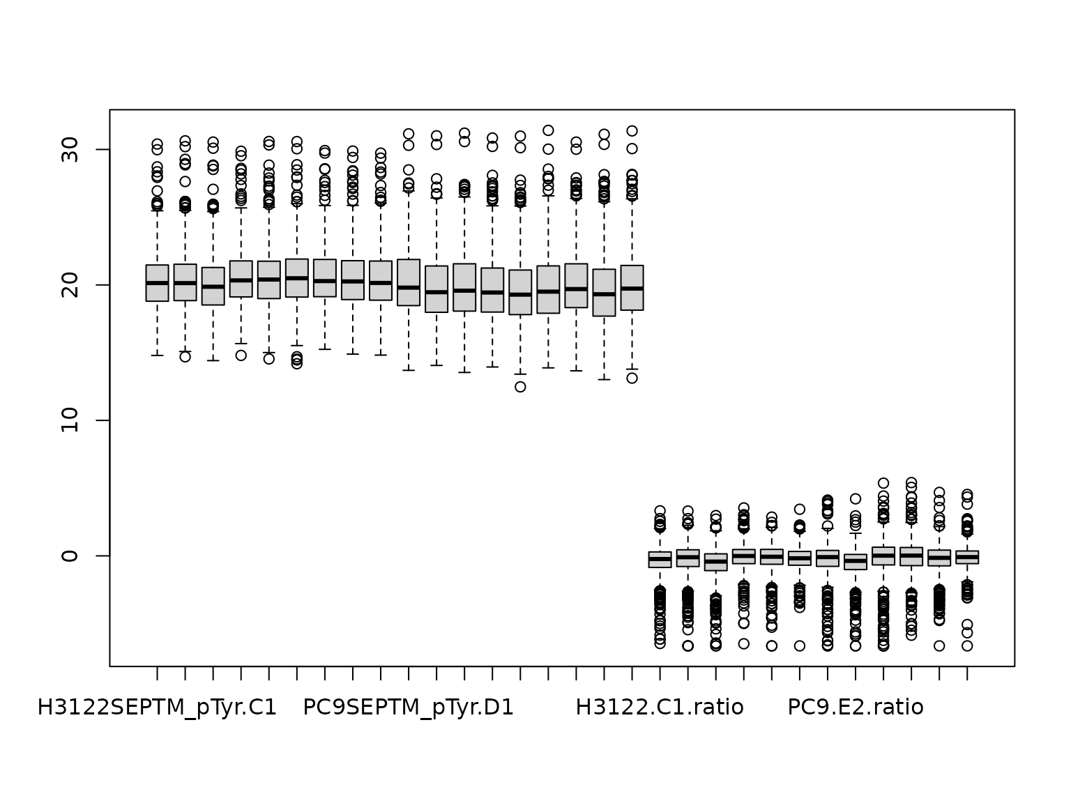

And do one more check:

identical(rownames(phos_ratios.lim.log2), rownames(log2phosdata)) 
>> [1] TRUE

This can be used as the example ptmtable for subsequent testing.

# ptmtable <- phosdata_plus_ratios

Combining data from multiple PTM experiments

For experiments involving multiple PTMs, or if investigators wish to combine several data sets, the data can be combined. For example, pulldowns were made to isolate acetylated and ubiquitinated peptides from the same experimental samples. Combining the data is simply repeating the above steps using the correct optimum data columns, then making the column names the same, and binding all the rows together.

Suppose you had acetylation data in ackdata.df and ubiquitination data in ubidata.df, both formatted as above for phosphorylation data in phosdata.df. You could combine them as follows.

First, make sure the column names are the same:

kgp <- phosdata.df
kga <- ackdata.df
kgu <- ubidata.df

names(kgp) <- sapply(names(kgp), function(x){
  paste(unlist(strsplit(x, "_pTyr"))[1], unlist(strsplit(x, "_pTyr"))[2],
        sep = "")
  })

names(kga) <- sapply(names(kga), function(x){
  paste(unlist(strsplit(x, "_AcK"))[1], unlist(strsplit(x, "_AcK"))[2],
        sep = "")
  })

names(kgu) <- sapply(names(kgu), function(x){
  paste(unlist(strsplit(x, "_Ubi"))[1], unlist(strsplit(x, "_Ubi"))[2],
        sep = "")
  })

identical(names(kgp), names(kga)) # Check TRUE

Then rbind them:

ptmdata <- rbind (kgp, kga, kgu)

Reorder:

ptmdata <- ptmdata[order(rownames(ptmdata)),]

This optional step improves clustering in our hands:

log2ptmdata <- log2(ptmdata)

Finally, this dataframe could be used as the example ptmtable for the P2P functions.

# ptmtable <- log2ptmdata

Lucia Williams, Nagashree Avabhrath, Mikhail Ukrainetz, Madison Moffett, Grant Smith, Mark Grimes