
Getting Started with PTMsToPathways
Nagashree Avabhrath, Mikhail Ukrainetz, Madison Moffett, Grant Smith, Lucia Williams, Mark Grimes
Source:vignettes/GettingStarted.Rmd
GettingStarted.RmdThis tutorial is intended to be a step-by-step guide to walk users through the main functions of the P2P package. It includes descriptions of each function and must be run in order as subsequent steps require the data produced in previous steps. For large datasets, it may be useful to save the output of each step to a file for later use.
Installation
Installation instructions for the P2P package can be found on the main package page.
Then load the package:
Starting Data
For the tutorial, we will be using two example datasets: a smaller dataset consisting of 933 PTMs and 18 experimental conditions (the example used in the Raw Data Processing vignette) and a larger dataset containing around 9000 PTMs and 69 experimental conditions. These datasets are available with the package. Alternatively, the larger dataset can be downloaded here to be inspected locally.
To see all data that is provided with the package, run:
data(package = "PTMsToPathways")| Dataset Name | Description |
|---|---|
| BRCA_PCN.data | BRCA PCN Data |
| BRCA_genemania.edges | BRCA Genemania Edges |
| BRCA_stringdb.edges | BRCA STRINGdb Edges |
| brca_CCCN_data | Output of MakeCorrelationNetwork on the BRCA data |
| brca_clusterlist_data | BRCA Cluster List Data |
| ex_PCNedgelist | PCN Edge List |
| ex_adj_consensus | Adjacency Consensus Matrix |
| ex_bioplanet | Bioplanet |
| ex_cfn | CFN |
| ex_combined_ppi | Combined PPIs |
| ex_common_clusters | Common Clusters |
| ex_full_ptm_table | Full PTM Table Example |
| ex_gene_cccn_edges | Gene CCCN Edgelist |
| ex_gene_cccn_nodes | Gene list (nodes) |
| ex_genemania_edges | Genemania Edges |
| ex_pathway_crosstalk_network | Pathway Crosstalk Network |
| ex_pathways_list | Pathways list |
| ex_ptm_cccn_edges | PTM CCCN Edgelist |
| ex_ptm_correlation_matrix | Correlation Matrix |
| ex_small_ptm_table | Small PTM Table Example |
| ex_stringdb_edges | STRINGdb Edges |
| ex_tiny_ptm_table | Tiny PTM Table Example |
| function_key | Function Key Example |
If you are using the smaller dataset, use the following code to view the dimensions of the dataset and a small portion of it:
dim(ex_small_ptm_table)
ex_small_ptm_table[38:50, 1:2]
>> [1] 908  18
>>                            H3122SEPTM_pTyr.C1 H3122SEPTM_pTyr.C2
>> HNRNPA3 p S358                             NA                 NA
>> EPHB4 p S575                               NA                 NA
>> BCAR1 p S407                           163730             159600
>> MAGOH p S38; MAGOHB p S40             1824100                 NA
>> DYNLL1 p S64; DYNLL2 p S64                 NA                 NA
>> PRKCD p S304                               NA                 NA
>> PCDH1 p S1018                              NA             563220
>> AHNAK p S5832                              NA                 NA
>> AHNAK p S5841                              NA                 NA
>> ARHGEF5 p S1139                            NA                 NA
>> SRSF9 p S178                               NA                 NA
>> RIPK1 p S389                               NA                 NA
>> URB2 p S18                                 NA                 NA
If you want to use the bigger dataset, the following code shows the dimensions and a snippet of the dataset:
dim(ex_full_ptm_table)
ex_full_ptm_table[38:50, 1:2]
>> [1] 9215   69
>>                                H3122SEPTM.C1 H3122SEPTM.C2
>> ABCC4 ubi K540                      20.03456            NA
>> ABCC4 ubi K622                            NA            NA
>> ABCC4 ubi K695                            NA            NA
>> ABCC4 ubi K77                             NA            NA
>> ABCC5 p Y10                               NA            NA
>> ABCD1 ubi K407; ABCD2 ubi K411            NA            NA
>> ABCD3 ack K260                            NA            NA
>> ABCD3 ubi K260                            NA            NA
>> ABCD3 ubi K576                            NA            NA
>> ABCE1 ubi K121                      17.62671      17.65533
>> ABCE1 ubi K210                            NA            NA
>> ABCE1 ubi K250                            NA            NA
>> ABCE1 ubi K93                             NA            NA
If you have downloaded the larger dataset locally, you can read it into R using the following code:
allptmtable <- utils::read.table("AlldataPTMs.txt", sep = "\t", skip = 0,
                                 fill = T, quote = "\"", dec = ".",
                                 comment.char = "", stringsAsFactors = F)
Using Your Own Data
To use your own MS data, you will need to transform it into a dataframe with PTMs and row names, experimental conditions as column names, and numeric data as the entries. Please refer to the Raw Data Processing vignette for a tutorial showing all steps needed to transform an MS output file into a P2P package input dataframe.
Step 1: Make Cluster List
MakeClusterList is the first step in the P2P process.
This function takes the dataframe ptmtable and runs it
through three calculations of statistical measures of distance:
Euclidean Distance, Spearman Dissimilarity (1- |Spearman Correlation|),
and SED (the average of both Spearman Dissimilarity (1- Spearman
Correlation) and Euclidean Distance). Combining the two dissimilarities
leads to better resolution of the data and is useful in pattern
recognition. A correlation table— ptm.correlation.matrix—is
generated based on the distances calculated for each pair of PTMs. The
function then runs the matrices through t-SNE to generate clusters based
on the previously calculated distance and provides you with a cluster
list, common.clusters. The returned
adj.consensus.matrix (which identifies which PTMs cluster
together with a ‘short distance’ between them) and
ptm.correlation.matrix are also used in the next step to
create co-cluster correlation networks (CCCNs). These three outputs are
returned as a list.
The keeplength paramter defines the minimum number of
PTMs that must be in a cluster for it to be retained in the final
output. The toolong parameter defines the maximum distance
between two PTMs for them to be considered as clustering together.
MakeClusterList can be run like so:
set.seed(88)
clusterlist.data <- MakeClusterList(ex_small_ptm_table,
                                    keeplength = 2, toolong = 3.5)
>> Starting correlation calculations and t-SNE.
>> This may take a few minutes or hours for large data sets.
>> Warning in stats::cor(t(ptmtable), use = "pairwise.complete.obs", method =
>> "spearman"): the standard deviation is zero
>> Warning in stats::cor(t(ptmtable), use = "pairwise.complete.obs", method =
>> "spearman"): the standard deviation is zero
>> Warning in stats::cor(t(ptmtable), use = "pairwise.complete.obs", method =
>> "spearman"): the standard deviation is zero
>> Warning in stats::cor(t(ptmtable), use = "pairwise.complete.obs", method =
>> "spearman"): the standard deviation is zero
>> Warning in stats::cor(t(ptmtable), use = "pairwise.complete.obs", method =
>> "spearman"): the standard deviation is zero
>> Warning in stats::cor(t(ptmtable), use = "pairwise.complete.obs", method =
>> "spearman"): the standard deviation is zero
>> Warning in stats::cor(t(ptmtable), use = "pairwise.complete.obs", method =
>> "spearman"): the standard deviation is zero
>> Warning in stats::cor(t(ptmtable), use = "pairwise.complete.obs", method =
>> "spearman"): the standard deviation is zero
>> Spearman correlation calculation complete after 12.13 secs total.
>> Spearman t-SNE calculation complete after 40.39 secs total.
>> Euclidean distance calculation complete after 40.44 secs total.
>> Euclidean t-SNE calculation complete after 1.11 mins total.
>> Combined distance calculation complete after 1.11 mins total.
>> SED t-SNE calculation complete after 1.56 mins total.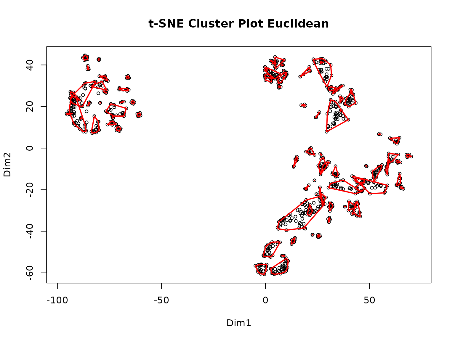
>> Clustering for Euclidean complete after 1.57 mins total.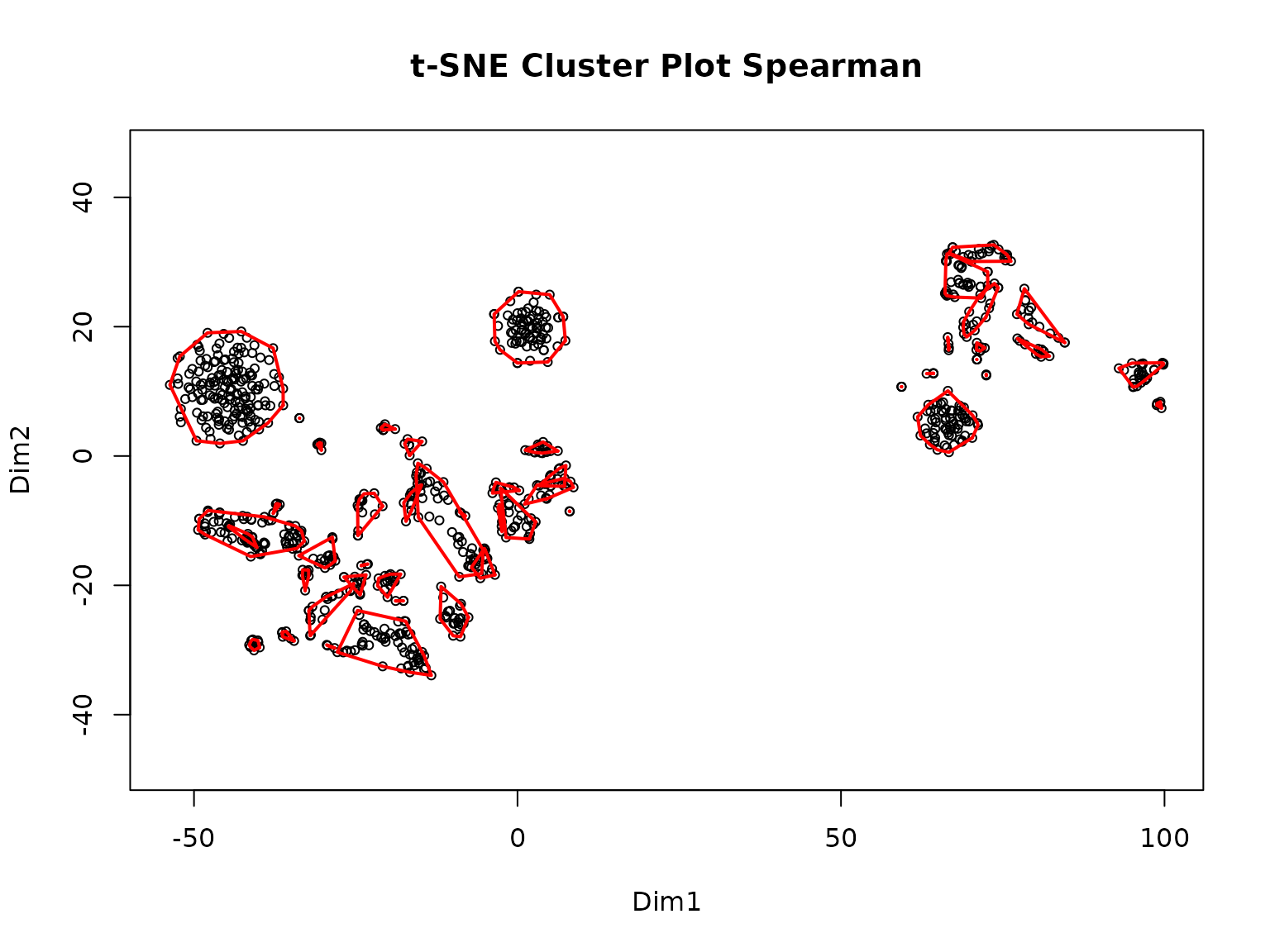
>> Clustering for Spearman complete after 1.57 mins total.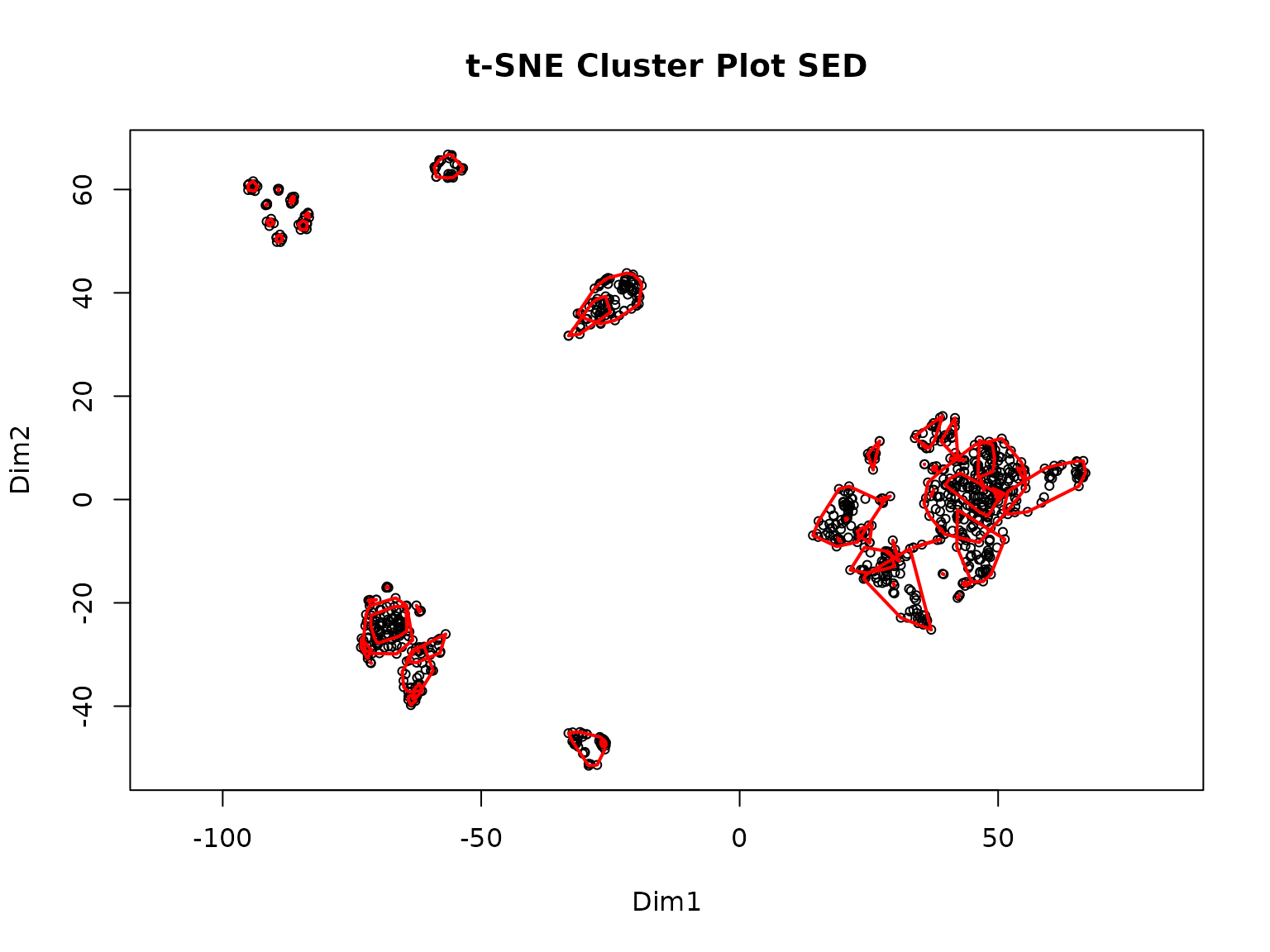
>> Clustering for SED complete after 1.58 mins total.
>> Consensus clustering complete after 1.58 mins total.
>> MakeClusterList complete after 1.58 mins total.
The following unpacks the output into the separate objects discussed above:
common.clusters <- clusterlist.data[[1]]
adj.consensus.matrix <- clusterlist.data[[2]]
ptm.correlation.matrix <- clusterlist.data[[3]]
Now we can view the objects. First, here is an example of a cluster:
common.clusters[1]
>> $ConsensusCluster1
>> [1] "KRT7 p S37"
>> [2] "CALM3 p Y100; CALM2 p Y100; CALM1 p Y100"
>> [3] "ERP29 p Y66"
>> [4] "MYH9 p Y1408"
>> [5] "PTK2 p Y925"
>> [6] "TNK2 p Y827"
>> [7] "ITSN2 p Y553"
>> [8] "PRRC2C p Y1218"
Next, we look at a piece of the adjacency matrix. Ones represent a pair that cluster and zeroes represent a pair that doesn’t:
adj.consensus.matrix[7:10, 7:10]
>>               CTNND1 p S225 CTNND1 p S230 STAM2 p S375 EGFR p S1166
>> CTNND1 p S225             0             0            0            0
>> CTNND1 p S230             0             0            0            0
>> STAM2 p S375              0             0            0            0
>> EGFR p S1166              0             0            0            0
Here is a part of the PTM correlation matrix. Values for pairs of PTMs are Spearman correlation coefficients ranging from -1 to 1. If two PTMs had no experimental conditions in common, their correlation value will be NA.
Step 2: Make Co-Cluster Correlation Networks (PTM and Gene)
The data generated in the previous step is next used to create a new network of PTMs that have strong associations called the Co-cluster Correlation Network (CCCN). The Spearman correlations between co-clustered PTMs are used as edge-weights in this network. The MakeCorrelationNetwork function groups the PTM correlation matrices by PTMs that co-cluster together to create a PTM CCCN. It then defines a relationship between proteins modified by PTMs and creates a gene CCCN with sum of the PTM correlations serving as edge weights.
CCCN.data <- MakeCorrelationNetwork(adj.consensus.matrix,
                                    ptm.correlation.matrix)
>> Making PTM CCCN
>> PTM CCCN complete after 0.06 secs total.
>> Making Gene CCCN
>> Gene CCCN complete after 2.77 secs total.
ptm.cccn.edges <- CCCN.data[[1]]
gene.cccn.edges <- CCCN.data[[2]]
gene.cccn.nodes <- CCCN.data[[3]]
We can view a portion of the PTM CCCN edges:
ptm.cccn.edges[18:22,]
>>           source        target     Weight          interaction
>> 18 EIF2B1 p S131   PKP4 p S273 -0.6833333 negative correlation
>> 19   LDHB p S238   EML4 p S242 -1.0000000 negative correlation
>> 20 S100A16 p S27   EML4 p S242 -0.5000000 negative correlation
>> 21     PXN p S90 S100A14 p S33 -0.3571429          correlation
>> 22    URB2 p S18 SHANK2 p S589  0.5428571 positive correlation
And a portion of the gene CCCN edges:
gene.cccn.edges[1:5,]
>>   source target     Weight          interaction
>> 1 ADGRL2  ALDOA -0.4535714          correlation
>> 2   ACP1    ALK  0.6000000 positive correlation
>> 3  AHNAK   ANO1  1.5428571 positive correlation
>> 4   ACP1  ANXA2 -0.2571429          correlation
>> 5 ADAM10  ANXA2  0.1702786          correlation
Finally, we can view a portion of the gene CCCN nodes, which are used to map to external PPI databases in the next step:
Because this step can take a long time to run on larger datasets, the output may be saved as an RData object for later use.
save.image(file = "filepath/name.RData")
# All objects in the environment are saved
Step 3: Retrieve Database Edgefiles
The third step of the P2P package is to gather data from multiple existing protein-protein interaction (PPI) databases which will be integrated with the data generated in steps 1 and 2. The P2P package explicitly allows the users to integrate data from three external databases: STRING, GeneMANIA, and PhosphoSite Plus. Other databases can also be downloaded and added to the PPI network. All three external databases have different interfaces for downloading data, so we show how to retrieve data from each of them below.
For this tutorial, we use the local STRING option so the vignette can
build offline. We also provide the option (using the switch
local = FALSE) to retrieve edges from STRINGdb online.
1. STRINGdb
STRINGdb can be queried directly
from R using the STRINGdb package. We wrap this query in a
function called GetSTRINGdb.edges, which queries only for
the genes found in clusters in previous steps, and filters the returned
by interaction type so only experimental,
database, experimental_transferred, and
database_transferred are retained. This ensures that only
interactions with more substantial evidence are used in this
analysis.
Alternatively, as shown below, the user can download a pre-processed STRINGdb file that can be used in place of the live online query. The data can be found on Zenodo. Here, we use a small subset of the data downloadable from Zenodo.
path <- system.file("extdata", "small_string_hs_hugo.tsv",
                    package = "PTMsToPathways")
stringdb.edges <- GetSTRINGdb.edges(gene.cccn.edges, gene.cccn.nodes, local=TRUE,
    string.local.path = path)
>> Reading local STRING file: /home/runner/work/_temp/Library/PTMsToPathways/extdata/small_string_hs_hugo.tsv
stringdb.edges[1:5,]
>>   source   target             interaction Weight
>> 1   ACLY   EIF4A1             experiments    334
>> 2   ACLY     GOT1                database    800
>> 3   ACLY HSP90AA1 experiments_transferred     70
>> 4   ACLY HSP90AB1 experiments_transferred     70
>> 5   ACLY     LDHA experiments_transferred    346
2. GeneMANIA
To our knowledge, no R package exists to programmatically query GeneMANIA. Thus, we recommend using the GeneMANIA Cytoscape App to retrieve PPI data as follows.
First, create an input file for GeneMANIA using the
MakeDBInput function provided within P2P (note that this
creates a text file in your working directory):
MakeDBInput(gene.cccn.nodes, file.path.name = "db_nodes.txt")Next, ensure that you have Cystoscape and the GeneMANIA extension installed.
Copy the contents of the db_nodes.txt file into the
GeneMANIA App’s “Genes of Interest” box and run query.
To save the results, click on the three lines in the upper right corner. This should be under the GeneMANIA side window beside the species. Click “Export Results”. The path to this file is the gm.results.path:
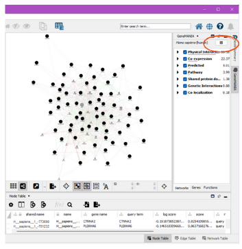
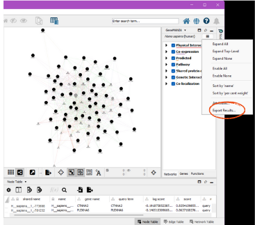
The GetGeneMANIA.edges function then processes the
output file produced by GeneMANIA itself. For example, we have saved
ex_gm_results.txt as an example output file from GeneMANIA
within the package. The following code shows how to use this file as
input to the function.
gm.results.path <- system.file("extdata", "ex_gm_results.txt",
                               package = "PTMsToPathways")
genemania.edges <- GetGeneMANIA.edges(gm.results.path, gene.cccn.nodes)
We can see an example of the GeneMANIA edges below:
3. Phosphosite Plus
The kinase-substrate data can be downloaded from Phosphosite Plus
database. The users will be required to create an account and sign in to
download the data. The GetKinsub.edges function reads this
downloaded data in and formats it so that all the PPI edge data frames
are in the same format for the next step.
input.filename <- system.file("extdata", "Kinase_Substrate_Dataset.txt",
                              package = "PTMsToPathways")
kinsub.edges <- GetKinsub.edges(input.filename,
                                  gene.cccn.nodes)
Step 4: Build PPI Network and Cluster Filtered Network
The BuildClusterFilteredNetwork function allows the
users to filter protein-protein interaction networks using the
previously generated co-cluster correlation networks. PPIs are retained
in the cluster filtered network (CFN) only if the interacting proteins
share statistically correlated PTMs identified via t-SNE clusters. The
BuildClusterFilteredNetwork function combines all the PPI
data downloaded in step 3 as efficiently as possible while retaining the
desired edge weights. It then normalizes the weights on a scale of 0-1
and gives an output cluster filter network that will only retain
interacting proteins whose genes are within the co-cluster correlation
network created in step 2.
We first run the function:
network.list <- BuildClusterFilteredNetwork(gene.cccn.edges,
                                            stringdb.edges,
                                            genemania.edges,
                                            kinsub.edges,
                                            db.filepaths = c())
And then unpack the outputs into separate variables:
combined.PPIs <- network.list[[1]]
cfn <- network.list[[2]]
We can view a portion of the CFN below:
cfn[1:5,]
>>   source target interaction Weight
>> 1   CDK1   CTTN          pp      1
>> 2   CDK1   EGFR          pp      1
>> 3   CDK1 HNRNPK          pp      1
>> 4   CDK1   KRT8          pp      1
>> 5   CDK1   LDHA          pp      1
To reduce clutter on graphs, the CFN edges can be merged. This collapses two or more edges between two nodes into a single edge, combining edge names:
cfn.merged <- mergeEdges(cfn)Step 5: Pathway Crosstalk Network
The final step is the creation of the Pathway Crosstalk Network
(PCN). This step requires input of an external database from NCATS
BioPlanet that contains groups of genes (proteins) involved in
various cellular processes known as pathways.
BuildPathwayCrosstalkNetwork turns this data file into a
list of pathways and converts those pathways into a list of
pathway-pathway edges, each of which is assigned a Jaccard similarity
and a Cluster-Pathway Evidence score based on the common clusters found
in the gene co-cluster correlation network. Info about the
Cluster-Pathway Evidence score can be found here
For graphing in Cytoscape, the Cluster-Pathway Evidence and Jaccard
similarity edges are listed separately in the edgelist called
pathway.crosstalk.network.
bioplanet.file <- system.file("extdata", "pathway.csv",
                              package = "PTMsToPathways")
The function BuildPathwayCrosstalkNetwork
takes the list of pathways (or a path to the pathway file) and the list
of clusters generated in step 1 and returns the relationships between
pathways in two forms: a dataframe of edges that can be uploaded to
Cytoscape (the first element of the returned list) and a dataframe with
columns for the two edge weights (the second element of the returned
list). The third element of the returned list is the list of pathways
(in case the user provided a path to the pathway file rather than a list
of pathways). The fourth element is the cluster-by-pathway CPE matrix
used for the PTM cluster weight calculations. The function can be run as
follows:
PCN.data <- BuildPathwayCrosstalkNetwork(common.clusters, bioplanet.file)
>> Making PCN
>> 2026-09-14 04:56:48.415522
>> 2026-09-14 04:56:48.534288
>> Total time: 0.11876654624939
pathway.crosstalk.network <- PCN.data[[1]]
PCNedgelist <- PCN.data[[2]]
pathways.list <- PCN.data[[3]]
CPE.matrix <- PCN.data[[4]]
If you want to save the Cytoscape-ready edgefile, save the returned
pathway.crosstalk.network dataframe explicitly:
utils::write.csv(pathway.crosstalk.network,
                 file = "PCN_file.csv",
                 row.names = FALSE)
The required columns for Cytoscape are:
And we can see some of the pathway crosstalk network edges below:
pathway.crosstalk.network[1:5,]| source | target | Weight | interaction | |
|---|---|---|---|---|
| 4 | Axon guidance | Validated nuclear estrogen receptor alpha network | 1.27898550724638 | PTM_cluster_weights |
| 2 | Axon guidance | ERBB signaling pathway | 9.50912807669002 | PTM_cluster_weights |
| 3 | Axon guidance | Lipid and lipoprotein metabolism | 4.63387820142684 | PTM_cluster_weights |
| 5 | ERBB signaling pathway | Lipid and lipoprotein metabolism | 2.96007824348337 | PTM_cluster_weights |
| 18 | Selenium pathway | Vitamin B12 metabolism | 0.866666666666667 | PTM_cluster_weights |
To understand the edge weights calculations, let’s consider a pair of
pathways, Axon Guidance and
ERBB signaling pathway. We’ll look at the
PCNedgelist dataframe this time.
PCNedgelist[PCNedgelist$source == "Axon guidance" & PCNedgelist$target == "ERBB signaling pathway", ]| source | target | pathway_Jaccard_similarity | PTM_cluster_weights | |
|---|---|---|---|---|
| 2 | Axon guidance | ERBB signaling pathway | 0.07 | 9.51 |
Pathway-pathway weight calculations
Jaccard Similarity
The Jaccard similarity is defined as the size of the intersection of the two pathways (the number of genes that are in both pathways) divided by the size of the union of the two pathways (the total number of unique genes that are in either pathway).
size_union <- length(union(pathways.list[["Axon guidance"]], pathways.list[["ERBB signaling pathway"]]))
size_intersection <- length(intersect(pathways.list[["Axon guidance"]], pathways.list[["ERBB signaling pathway"]]))
jaccard_similarity <- size_intersection / size_union
jaccard_similarity
>> [1] 0.07161125
Notice that the found value is the same as the
pathway_Jaccard_similarity value in the
PCNedgelist dataframe.
PTM Cluster Weight
P2P also calculates a PTM cluster based weight between pathways
(pathway_cluster_weight).
For a given pathway () and a given cluster (), we define the Cluster-Pathway Evidence (CPE), where is a protein in pathway and is a PTM.
(Note that means “in” and means “and”.)
Let’s break down the CPE calculation single cluster
,
the first cluster found, and a single pathway
,
the Axon guidance pathway.
c_i <- common.clusters[[1]]
p_j <- pathways.list[["Axon guidance"]]
length(c_i)
length(p_j)
>> [1] 8
>> [1] 325
Notice that the numerator of the summands in
counts the number of PTMs that are in both the protein and the cluster.
Intuitively, if a pathway contains many proteins that have PTMs in this
cluster, then this sum will be larger. Of the 325 proteins in the
Axon guidance pathway, only MYH9 and
PTK2 have PTMs that occur in the first cluster, so out of
the 325 summands in
,
only two are non-zero. And in fact, both numerators are 1, since there
is only one PTM on MYH9 in our cluster:
And also only one PTM onPTK2:
The denominators of the summands in
are the product of the number of pathways that the protein is in and the
number of PTMs in the cluster. From above, there are 8 PTMs in this
cluster. MYH9 is in 1 pathway and PTK2 is in 2
pathways, as seen below:
sum(sapply(pathways.list, function(x) "MYH9" %in% x))
sum(sapply(pathways.list, function(x) "PTK2" %in% x))
>> [1] 1
>> [1] 2
(Note that the pathways.list here is a smaller version
of the full BioPlanet pathways list.)
So CPE for the first cluster and the Axon guidance
pathway is:
We can see that this is the same value as the CPE score for the first
cluster and the Axon guidance pathway in the
CPE.matrix:
Overall, two pathways are considered to be related if they both have positive CPE with at least one cluster. In that case, the PTM cluster weight for the two pathways is the sum of the CPE scores for all clusters that have positive CPE with both pathways. So if a cluster has positive CPE with both pathways, it contributes to the PTM cluster weight between those two pathways.
For the Axon guidance and
ERBB signaling pathway pair, we can see all of those
clusters and their CPE scores with both pathways in the
CPE.matrix:
cols <- c("Axon guidance", "ERBB signaling pathway")
rows <- rowSums(!is.na(CPE.matrix[, cols])) == 2
CPE.matrix[rows, cols]| Axon guidance | ERBB signaling pathway | |
|---|---|---|
| ConsensusCluster1 | 0.19 | 0.06 |
| ConsensusCluster2 | 0.07 | 0.07 |
| ConsensusCluster6 | 0.12 | 0.12 |
| ConsensusCluster7 | 0.12 | 0.12 |
| ConsensusCluster8 | 0.19 | 0.06 |
| ConsensusCluster9 | 0.21 | 0.07 |
| ConsensusCluster10 | 0.05 | 0.22 |
| ConsensusCluster12 | 0.15 | 0.05 |
| ConsensusCluster20 | 0.19 | 0.06 |
| ConsensusCluster21 | 0.05 | 0.15 |
| ConsensusCluster22 | 0.07 | 0.06 |
| ConsensusCluster26 | 0.12 | 0.12 |
| ConsensusCluster35 | 0.05 | 0.05 |
| ConsensusCluster36 | 0.07 | 0.04 |
| ConsensusCluster41 | 0.08 | 0.08 |
| ConsensusCluster43 | 0.15 | 0.03 |
| ConsensusCluster46 | 0.12 | 0.12 |
| ConsensusCluster49 | 0.05 | 0.05 |
| ConsensusCluster50 | 0.19 | 0.06 |
| ConsensusCluster55 | 0.17 | 0.17 |
| ConsensusCluster56 | 0.17 | 0.17 |
| ConsensusCluster60 | 0.17 | 0.17 |
| ConsensusCluster61 | 0.50 | 0.17 |
| ConsensusCluster69 | 0.07 | 0.07 |
| ConsensusCluster70 | 0.11 | 0.03 |
| ConsensusCluster78 | 0.10 | 0.10 |
| ConsensusCluster80 | 0.20 | 0.20 |
| ConsensusCluster81 | 0.10 | 0.10 |
| ConsensusCluster82 | 0.09 | 0.04 |
| ConsensusCluster87 | 0.12 | 0.25 |
| ConsensusCluster96 | 0.12 | 0.12 |
| ConsensusCluster97 | 0.38 | 0.12 |
| ConsensusCluster103 | 0.18 | 0.04 |
| ConsensusCluster116 | 0.30 | 0.10 |
| ConsensusCluster130 | 0.50 | 0.50 |
And the total is the same as the pathway_cluster_weight
for this pair above.
For more detail on the PTM cluster weight calculation, see “Ross et al., 2023”.
Saving Data
If you want to save your data to a file, all data structures can either be exported with the save function and loaded later or saved to a csv file with the write.csv function.
To save one object:
save(object, filename = "filepath/name.rda") # Saves object as an .rda
load("filepath/name.rda")                    # Loads object saved to a file
For multiple objects: Note the objects are saved as an .RData rather than an .rda
save(object1, object2, object.ect, filename="NewFile.RData")To save one object as a csv:
utils::write.csv(object, file = "filepath/name.csv") # Saves object as a .csv
utils::read.csv(file = "filepath/name.csv")          # Loads object from .csv
You may also save your entire Global Environment namespace using the save.image function as shown below:
save.image(file = "filepath/name.RData")
# All objects in the environment are saved
Session Info
sessionInfo()
>> R version 4.6.1 (2026-06-24)
>> Platform: x86_64-pc-linux-gnu
>> Running under: Ubuntu 24.04.5 LTS
>>
>> Matrix products: default
>> BLAS:   /usr/lib/x86_64-linux-gnu/openblas-pthread/libblas.so.3
>> LAPACK: /usr/lib/x86_64-linux-gnu/openblas-pthread/libopenblasp-r0.3.26.so;  LAPACK version 3.12.0
>>
>> locale:
>>  [1] LC_CTYPE=C.UTF-8       LC_NUMERIC=C           LC_TIME=C.UTF-8
>>  [4] LC_COLLATE=C.UTF-8     LC_MONETARY=C.UTF-8    LC_MESSAGES=C.UTF-8
>>  [7] LC_PAPER=C.UTF-8       LC_NAME=C              LC_ADDRESS=C
>> [10] LC_TELEPHONE=C         LC_MEASUREMENT=C.UTF-8 LC_IDENTIFICATION=C
>>
>> time zone: UTC
>> tzcode source: system (glibc)
>>
>> attached base packages:
>> [1] stats     graphics  grDevices utils     datasets  methods   base
>>
>> other attached packages:
>> [1] PTMsToPathways_0.99.0
>>
>> loaded via a namespace (and not attached):
>>  [1] Matrix_1.7-5      jsonlite_2.0.0    dplyr_1.2.1       vegan_2.7-6
>>  [5] compiler_4.6.1    tidyselect_1.2.1  Rcpp_1.1.2        parallel_4.6.1
>>  [9] cluster_2.1.8.2   jquerylib_0.1.4   splines_4.6.1     systemfonts_1.3.2
>> [13] textshaping_1.0.5 yaml_2.3.12       fastmap_1.2.0     lattice_0.22-9
>> [17] R6_2.6.1          plyr_1.8.9        generics_0.1.4    igraph_2.3.3
>> [21] knitr_1.52        MASS_7.3-65       tibble_3.3.1      Rtsne_0.17
>> [25] desc_1.4.3        pillar_1.11.1     bslib_0.12.0      rlang_1.3.0
>> [29] cachem_1.1.0      xfun_0.60         fs_2.1.0          sass_0.4.10
>> [33] otel_0.2.0        cli_3.6.6         withr_3.0.3       magrittr_2.0.5
>> [37] pkgdown_2.2.1     mgcv_1.9-4        digest_0.6.39     grid_4.6.1
>> [41] permute_0.9-10    lifecycle_1.0.5   nlme_3.1-169      vctrs_0.7.3
>> [45] glue_1.8.1        evaluate_1.0.5    ragg_1.5.2        rmarkdown_2.32
>> [49] purrr_1.2.2       pkgconfig_2.0.3   tools_4.6.1       htmltools_0.5.9